Realistic LES: the cabauw case

Generating input data using (LS) ² D

Download the data

To generate input based on ERA5, the (LS) ² D python package can be used. General instructions on (LS) ² D can be found here: https://github.com/LS2D/LS2D and a more elaborate description is given in the reference paper (van Stratum et al., 2023). ERA5 is described in Hersbach et al., (2020) and CAMS in Inness et al (2019). This tutorial shortly describes the steps to take and where to find the relevant scripts and functions.

1. Download the ERA5 (and CAMS) data.

This is done with the download_era5 function (and the download_cams function).

2. Read the data.

This is done with the Read_era5 class (and the Read_cams class). For the ERA5 data, this class also calculates some derived quantities such as thl.

3. Calculate large scale forcings.

This is done with the calculate_forcings function from the Read_era5 class that was called under step 2.

4. Interpolate the ERA5 and CAMS data to the MicroHH grid

This can be done with the get_les_input function from the Read_era5 class that was called under step 2 (and the get_les_input function from the Read_cams class).

5. Save the input variables to NetCDF.

Examples of python scripts that follow these steps are available.

For ERA5: https://github.com/LS2D/LS2D/blob/main/examples/example_era5.py

For CAMS: https://github.com/LS2D/LS2D/blob/main/examples/example_cams.py

Example

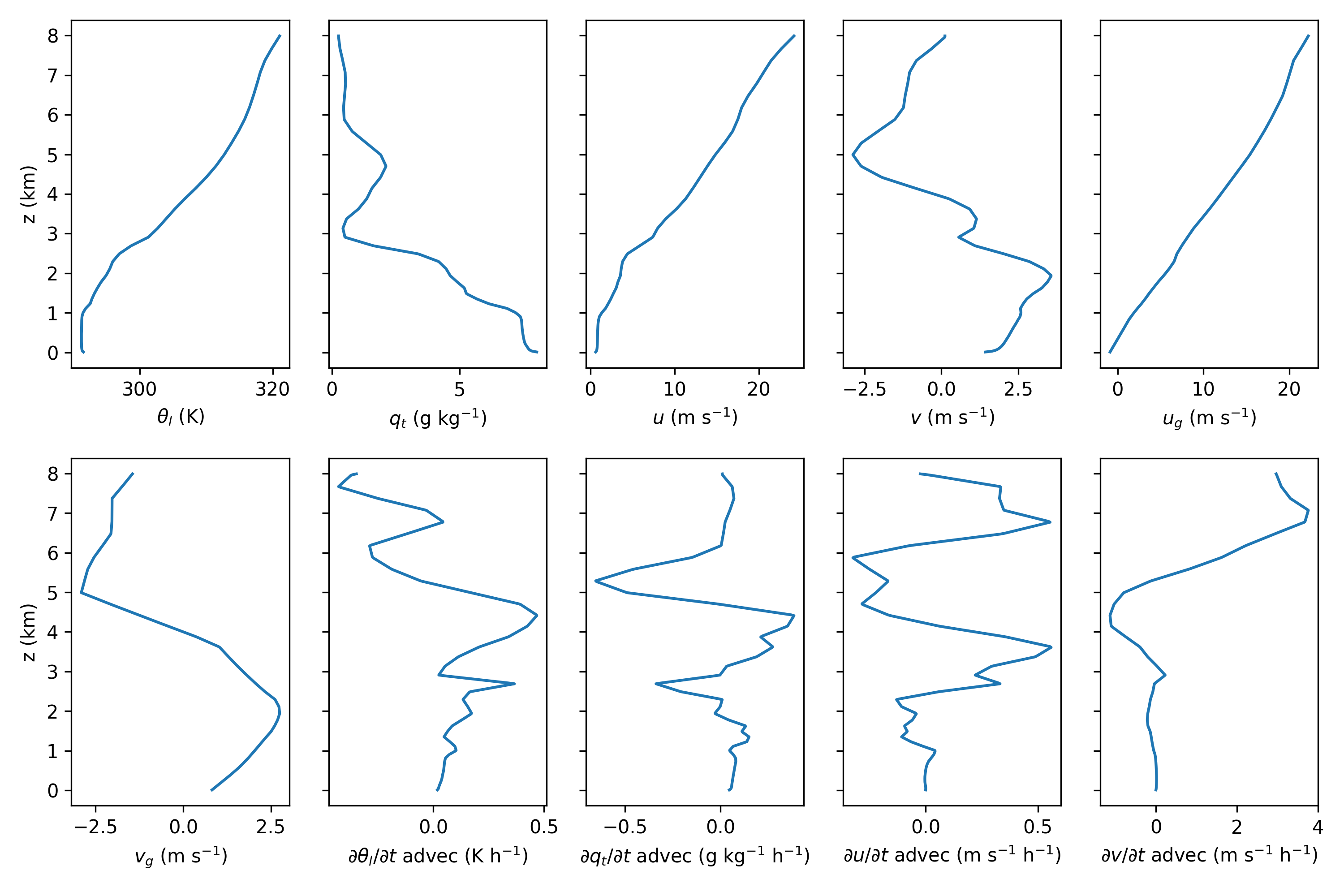
The plot below shows vertical profiles taken and derived from ERA5 using example_era5.py. This example shows 13 UTC on 4 July 2016.

Example

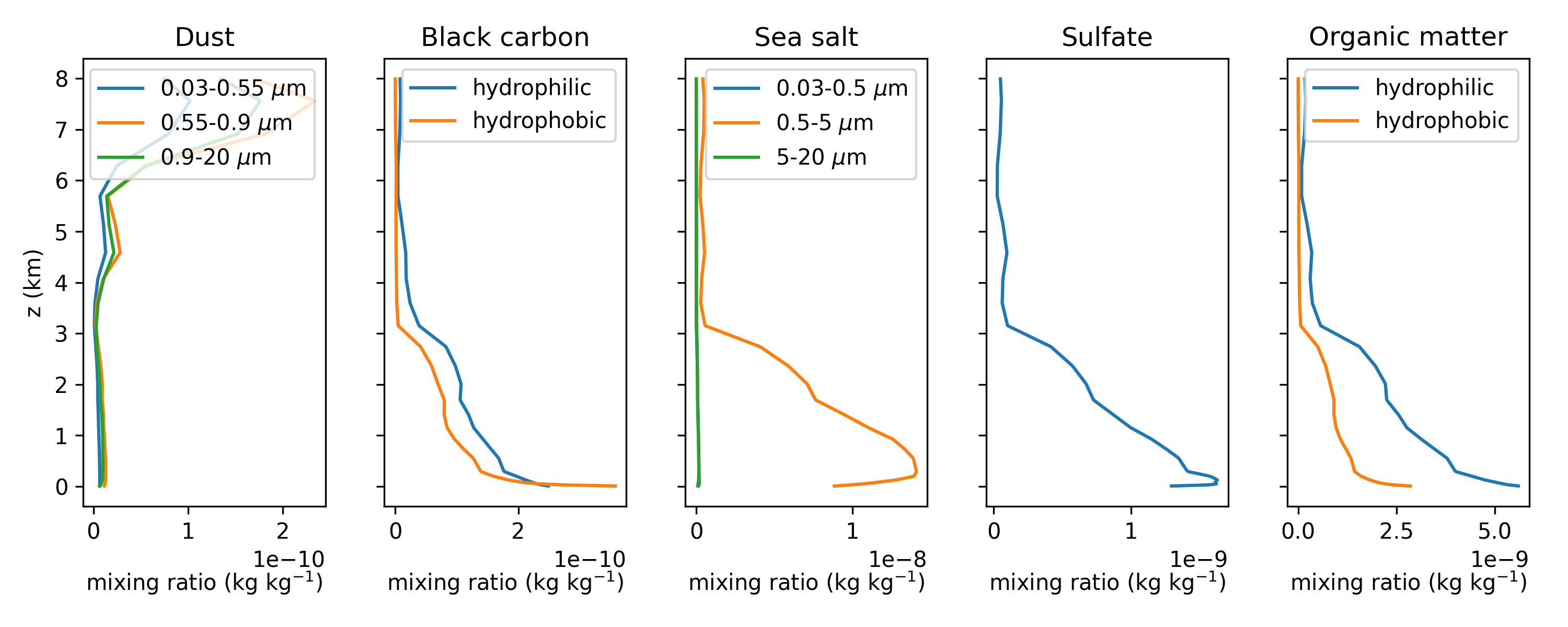
The plot below shows vertical profiles of aerosols mass mixing ratios taken from CAMS using example_cams.py. This example shows 13 UTC on 4 July 2016.

Note

1. When using CDS and ADS the $HOME/.cdsapirc file must contain the url and key for CDS as url and key and for ADS as url_ads and key_ads.

2. In example_cams.py and example_era5.py specify your own directories.

3. Optionally, specify your own date, time and location in the settings dictionary in example_cams.py and example_era5.py.

4. example_cams.py and example_era5.py stop after the download requests are submitted. Run them again once the data is downloaded to obtain the derived data.

5. Optionally, adapt the domain height in example_cams.py and example_era5.py. This must be larger than the desired domain height of the MicroHH simulation.

Creating input for MicroHH

The obtained files (ls2d_era5.nc and ls2d_cams.nc) can now be used to generate a yourcase_input.nc file. An example script to do this is available in /cases/cabauw/cabauw_input.py

The cabauw_input.py is a very complete script that allows to set many options that are discussed in the rest of this tutorial. It does not only produce cabauw_input.nc, it also produces cabauw.ini from cabauw.ini.base. Hence all the switches are set automatically, based on the flags given in cabauw_input.py. The code snippet below shows the part of cabauw_input.py where the flags are set.

"""
Case switches.
"""
TF = np.float64              # Switch between double (float64) and single (float32) precision.
use_htessel = True           # False = prescribed surface H+LE fluxes from ERA5.
use_rrtmgp = True            # False = prescribed surface radiation from ERA5.
use_rt = False               # False = 2stream solver for shortwave down, True = raytracer.
use_homogeneous_z0 = True    # False = checkerboard pattern roughness lengths.
use_homogeneous_ls = True    # False = checkerboard pattern (some...) land-surface fields.
use_aerosols = False         # False = no aerosols in RRTMGP.
use_tdep_aerosols = False    # False = time fixed RRTMGP aerosol in domain and background.
use_tdep_gasses = False      # False = time fixed ERA5 (o3) and CAMS (co2, ch4) gasses.
use_tdep_background = False  # False = time fixed RRTMGP T/h2o/o3 background profiles.

sw_micro = '2mom_warm'

"""
NOTE: `use_tdep_aerosols` and `use_tdep_gasses` specify whether the aerosols and gasses
      used by RRTMGP are updated inside the LES domain. If `use_tdep_background` is true, the
      aerosols, gasses, and the temperature & humidity are also updated on the RRTMGP background levels.
"""

# Switch between the two default RRTMGP g-point sets.
gpt_set = '128_112' # or '256_224'

# Time period.
# NOTE: Included ERA5/CAMS data is limited to 2016-08-15 06:00 - 18:00 UTC.
start_date = datetime(year=2016, month=8, day=15, hour=6)
end_date   = datetime(year=2016, month=8, day=15, hour=18)

# Simple equidistant grid.
zsize = 4000
ktot = 160

itot = 512
jtot = 512

xsize = 25600
ysize = 25600

In this part of the script, you can specify:

- the precision (TF)

- the start and end date/time (start_date, end_date)

- the domain size (zsize, xsize, y_size)

- the number of grid points (ktot, itot, jtot)

- settings regarding the land surface model (use_htessel, use_homogeneous_z0, use_homogeneous_ls) as discussed below (Land surface)

- setting regarding the radiation (use_rrtmgp, use_rt, use_aerosols, use_tdep_aerosols, use_tdep_gasses, use_tdep_background) as discussed below (Radiation)

- the microphysics scheme as discussed for the idealized cases (Microphysics)

Note

1. in cabauw_input.py, the filenames for the ERA5 and CAMS data must be specified.

2. currently, cabauw_input.py requires a file with the CAMS data, also if this data is not used.

Note

When running cabauw_input.py outside of the microhh directory be aware of the following:

1. cabauw.ini.base and microhh_tools.py must be present in the working directory.

2. the paths to the required lookup tables must be specified.

Large scale forcings

Our Cabauw simulation includes Large-scale forcings [force] based on ERA5. This includes the following aspects and their settings in cabauw.ini and cabauw_input.nc:

1. A large scale pressure force, derived from the time dependent geostropic wind and the coriolis parameter.

cabauw.ini: swlspres=geo, swtimedep_geo=true and fc=0.000115.

cabauw_input.nc: profiles of the geostropic wind (u and v) in the timedep group.

2. Time dependent large scale advection of thl, qt, u and v.

cabauw.ini: swls=1, swtimedep_ls=true, lslist=thl,qt,u,v and timedeplist_ls=thl,qt,u,v.

cabauw_input.nc: profiles of thl_ls, qt_ls, u_ls and v_ls in the timedep group.

3. Time dependent large scale subsidence based on the local field.

cabauw.ini: swwls=local and swtimedep_wls=true.

cabauw_input.nc: w_ls profile in the timedep group.

4. Nudging towards the time dependent ERA5 profiles of thl, qt, u and v.

cabauw.ini: swnudge=true, swtimedep_nudge=true and nudgelist=thl,qt,u,v.

cabauw_input.nc: profiles of thl_nudge, qt_nudge, u_nudge and v_nudge in the timedep group + profile of the nudging factor in the init group.

The cabauw_input.nc file also contains the time at which the time dependent variables are given.

Example

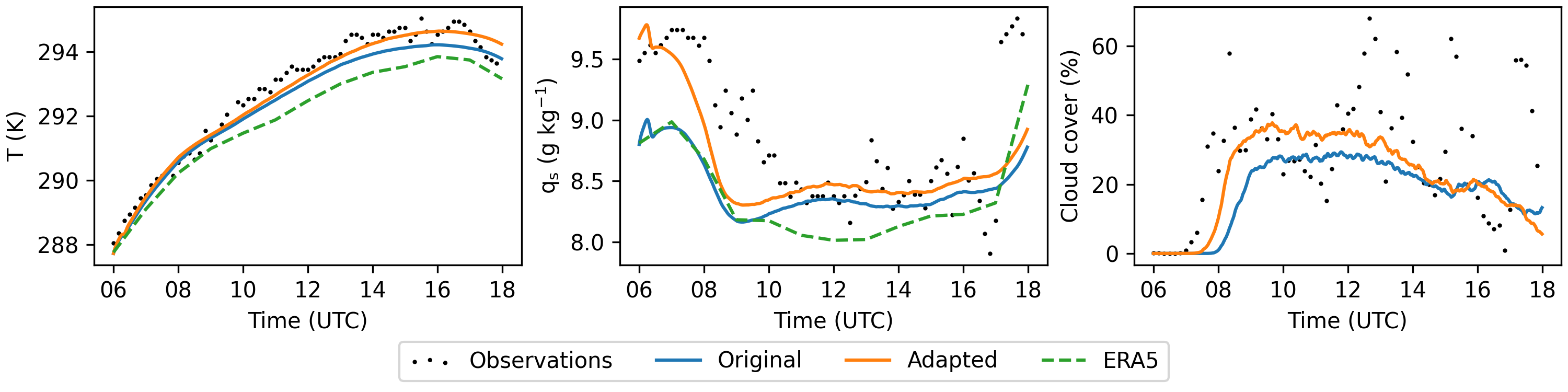
In cases where there is a mismatch between ERA5 and observations, a better match between MicroHH and observations can sometimes be obtained by manually tweaking the input profiles. An example is shown in the plot below for 4 July 2016, which shows timeseries of temperature and humidity at 10 m height and cloud cover. A better match with observations is realized by increasing the initial humidity with 10% at the surface, and a linearly decreasing percentage above until 1,000 m and by increasing the nudging timescale from 3 to 12 hr in the lowest 2 km.

Land surface

Our Cabauw simulation includes a surface model with an interactive land-surface scheme (Boundary conditions [boundary]). This scheme is similar to HTESSEL (Balsamo et al., 2019) The use of this scheme is specified in the cabauw.ini file by swboundary=surface_lsm and the settings in the [land_surface] group. The cabauw_input.nc file contains a soil group with profiles (of size ktot) of the soil temperature, soil water content, soil type, root fraction and depth of the soil layers.

Note

The interactive land-surface scheme can only be used in combination with swthermo=moist and swradiation = prescribed, rrtmgp or rrtmgp_rt

Note

The file van_genuchten_parameters.nc should be in the directory in which the model is run if [boundary][swboundary] = surface_lsm. This file can be found in /misc/van_genuchten_parameters.nc.

Example

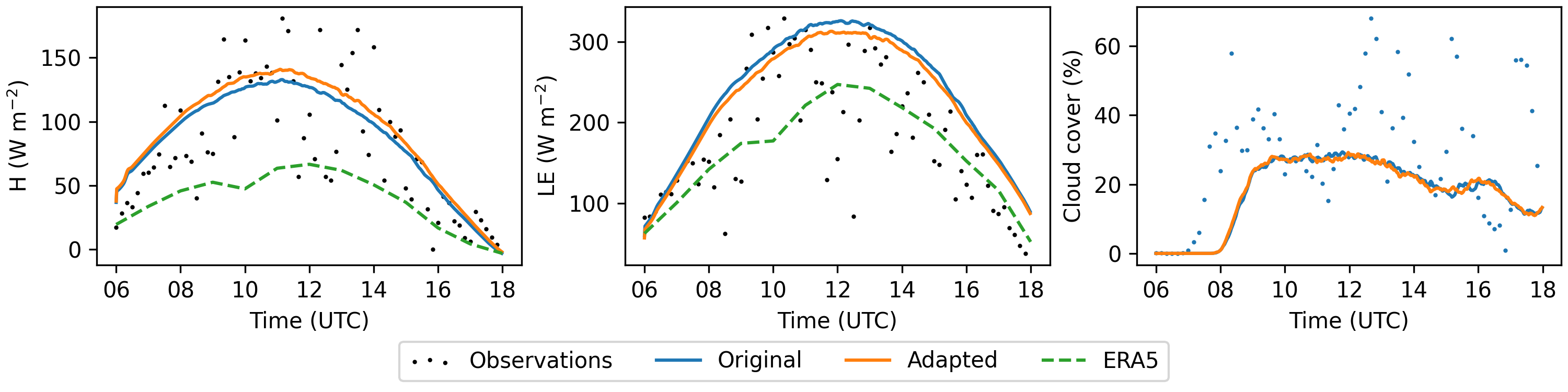
As with the initial conditions and large scale forcing, a better match wth observations can sometimes be obtained by manually tweaking the soil moisture content. An example is shown below for 4 July 2016 with a 10% reduction in soil moisture.

Radiation

Our Cabauw case includes Radiation [radiation] calculated with RTE+RRTMGP (Pincus et al., 2019). The C++ implementation of the code can be found here: https://github.com/microhh/rte-rrtmgp-cpp

The use of the radiation scheme is specified in cabauw.ini by swradiation=rrtmgp. Furthermore, cabauw.ini specifies the surface albedos for the direct and diffuse radiation (sfc_alb_dir, sfc_alb_dif), the surface emissivity (emis_sfc) and the radiation time interval (dt_rad). In addition, the Cabauw case uses a variable solar zenith angle, hence swfixedsza=false and therefore the latitude and longitude need to be specified in the grid group.

The cabauw_input.nc file contains a radiation group with profiles of height, temperature, pressure, H₂O, and O₃ at the ERA5 model levels. These profiles are used for calculating radiation in a background column. This is one column in which radiation is calculated to determine the incoming radiation at the top of the domain. This is necessary as the domain top is generally far below the top of the atmosphere, hence we need to account for the attenuation of radiation.

Furthermore, the init group of cabauw_input.nc contains concentrations of H₂O and O₃ at the model levels, for the radiation computations within the domain. The concentration of H₂O is only used initially, afterwards the simulated concentration is used.

Note

In general, concentration of a number of gasses must be provided for the radiation computations, either as a profile or as a constant. These gasses are at least H₂O, O₃, N₂O, O₂, CO₂, CH₄, and optionally also CO, N₂, CCl₄, CFC-11, CFC-12, CFC-22, HFC-143a, HFC-125, HFC-23, HFC-32, HFC-134a, CF₄, NO₂

Note

The _input.nc file will contain additional profiles when switching flags in cabauw_input.py to use time dependent gasses (use_tdep_gasses = True), time dependent background profiles (use_tdep_background=true), constant aerosols (use_aerosol=true and use_tdep_aerosols=false), and/or time dependent aerosols (use_aerosol=true and use_tdep_aerosols=false).

Apart from the _input.nc and .ini, additional files are required when using rrtmgp. The table below gives an overview of available lookup tables that should be present in the directory in which the model is run.

File name	Location of the file
coefficients_lw.nc	/rte-rrtmgp-cpp/rrtmgp-data/rrtmgp-gas-lw-g256.nc or /rte-rrtmgp-cpp/rrtmgp-data/rrtmgp-gas-lw-g128.nc
coefficients_sw.nc	/rte-rrtmgp-cpp/rrtmgp-data/rrtmgp-gas-sw-g224.nc or /rte-rrtmgp-cpp/rrtmgp-data/rrtmgp-gas-sw-g112.nc
cloud_coefficients_lw.nc	/rte-rrtmgp-cpp/rrtmgp-data/rrtmgp-clouds-lw.nc
cloud_coefficients_sw.nc	/rte-rrtmgp-cpp/rrtmgp-data/rrtmgp-clouds-sw.nc
aerosol_optics.nc	/rte-rrtmgp-cpp/data/aerosol_optics.nc

For the lookup tables coefficients_lw.nc and coefficients_sw.nc there are two files available with different numbers of g-points. Using less g-points is slightly less accurate, but requires less memory. The aerosol_optics.nc file is only required when aerosols are included.

Example

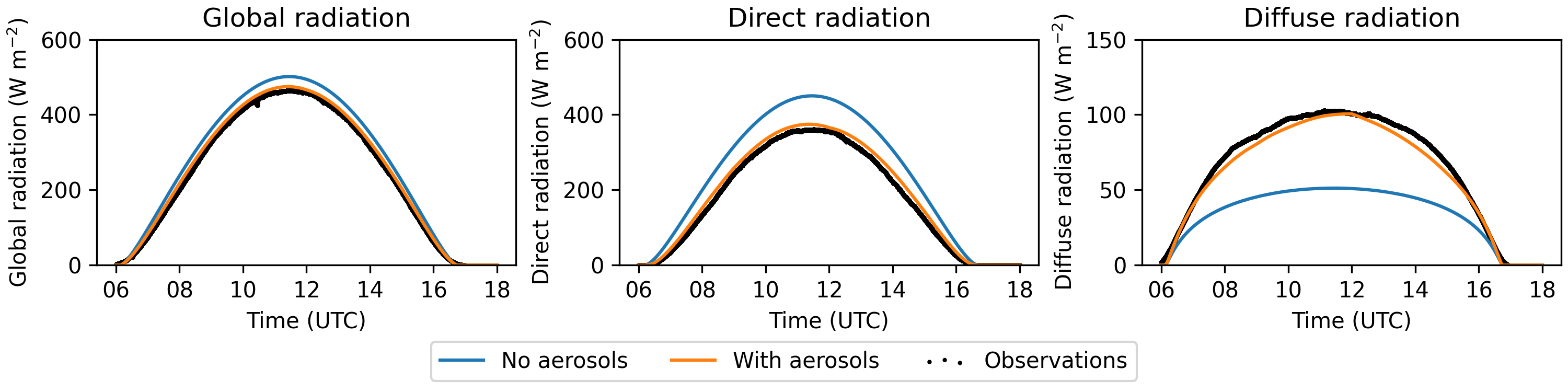
The figure below shows the components of surface radiation on 15 October 2017 with and without aerosols.

Ray tracing

Instead of the commonly used 2D radiative transfer calculations, MicroHH can also be ran with a coupled ray tracer (Veerman et al., 2022) to simulate radiation in 3D. The code, as well as some basic instructions can be found on https://github.com/microhh/rte-rrtmgp-cpp.

To use ray tracing coupled to a MicroHH simulation set swradiation=rrtmgp_rt in the .ini file. Additionally, the ray tracer uses a null-collision grid, which is a technique to divide the domain into smaller piece for efficient calculations. For any simulation with the ray tracer, the size of this grid in the three dimensions has to be specified in the .ini file (kngrid_i, kngrid_j, kngrid_k). In addition, the .ini file must contain the number of rays per pixel (rays_per_pixel), which must always be a power of 2. The most common values for rays per pixel are 64, 128 or 256, with the smaller numbers being faster but slightly less accurate.

Example

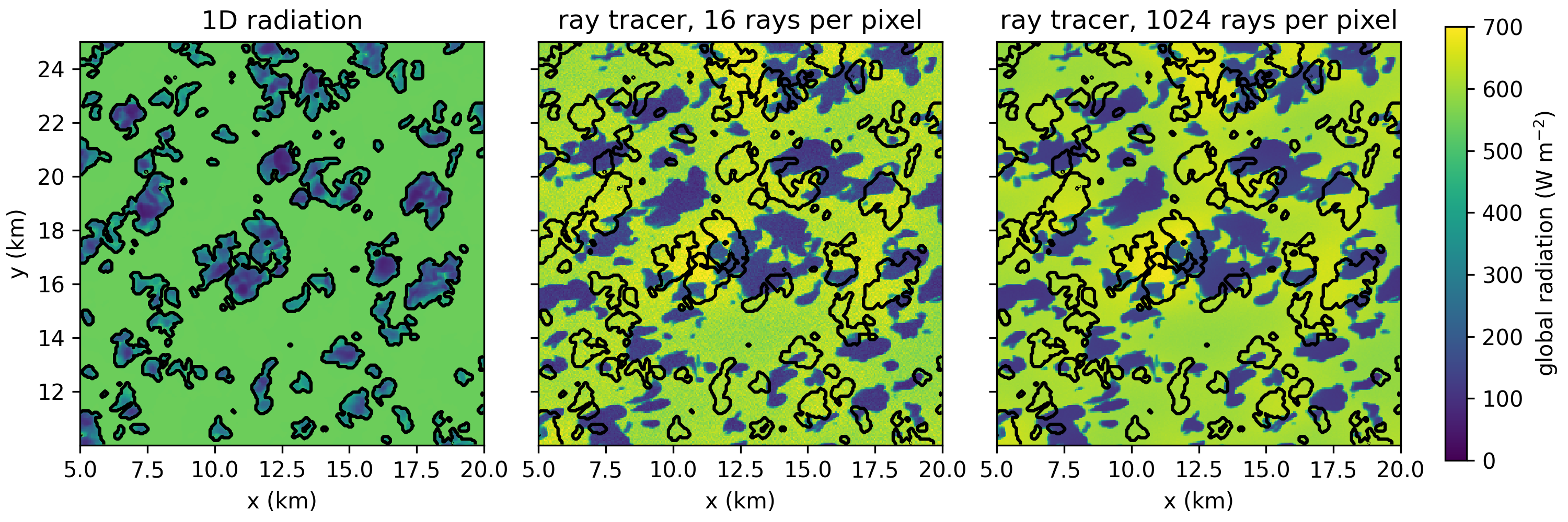
The figure below shows global radiation at the surface in colors and the cloud contours in black. The figure highlights the difference between 1D and 3D radiation and the difference between 16 and 1024 rays per pixel. The cloud field is taken from a simulation with 1D radiation on 4 July 2016 16 UTC.

Note

1. Currently, ray tracing is only available for shortwave radiation, requires an equidistant grid structure, and runs only on GPU.

2. column statistics are not available when using the coupled ray tracer.

It is also possible to run the ray tracer offline. In other words, to apply 3D radiative transfer calculations to a cloud field from a simulation with simpler radiation. Building the stand alone ray tracer is similar to building MicroHH and generates (among others) the executable test_rte_rrtmgp_rt_gpu.

Running the standalone ray tracer requires 3D fields of absolute temperature, specific humidity, cloud water content, ice water content and the essential gasses as listed above. In addition, a 3D grid is required, vertical profiles of density and pressure, and values for the surface albedo, surface emissivity, solar zenith angle, solar azimuth angle. Optionally, other gasses and aerosols can be added. To convert MicroHH output to input for the standalone ray tracer, a python script is available /python/microhh_to_raytracer_input.py. All available command line options are listed in the code for the forward ray tracer

Note

The standalone ray tracer can also be used for backward raytracing (tracing rays back from the surface upwards to compute radiances) with the executable test_rte_rrtmgp_bw_gpu

- The backward ray tracer requires additional information on the camera settings, which can be added with a python script /rte-rrtmgp-cpp/python/set_virtual_camera.py

- To visualize the output of the backward ray tracer, a python script is available /rte-rrtmgp-cpp/python/image_from_xyz.py

- All available command line options are listed in the code for the backward ray tracer.